
I am researcher working on robust Military Communication Systems.
This post will introduce the core concepts underlying various policy gradient algorithms. As opposed to previously introduced methods - which suffered from the curse of dimensionality - it is not necessary to analyze the full action space to update the policy \(\pi \) . These algorithms are an approach to reinforcement learning utilizing stochastic gradient ascent.
The Goal
Those of you familiar with neural networks will probably have heard of stochastic gradient descent. The goal of stochastic gradient descent is to compute the gradient of a loss function to then adjust the parameters of the network and minimize the loss function by stepping in the opposite direction of the gradient.
We can utilize the very similar stochastic gradient ascent to approach reinforcement learning problems. To this end, we define a reward function \(J(\theta)\) measuring the quality of our policy \(\pi_{\theta}\). In reinforcement learning this is quite simple since reinforcement inherently utilizes rewards $r$. Thus, the reward function is chosen to be the expected reward of a trajectory \(\tau\) generated by the current policy \(\pi_{\theta}\). Let \(G(\tau)\) be the infinite horizon discounted-return starting at time step \(t = 0\) for the trajectory \(\tau\).
The derivation of the policy gradient using finite or undiscounted returns are almost identical. For finite horizon $T$ simply replace all \(\infty\) with $T$.
$$ G(\tau) = \sum_{t = 1}^\infty \gamma^t r_{t+1} \ J(\theta) = \mathop{\mathbb{E}}_{\tau \sim \pi_\theta} [ G(\tau) ] $$
If it is possible to now calculate the gradient of the reward function /latex we can take a stochastic gradient ascent step based on a hyperparameter \(\alpha\) to maximize the reward function:
$$\theta = \theta + \alpha \nabla_\theta J(\theta) $$
The only problem remaining is to determine what the gradient \(\nabla_\theta J(\theta)\) looks like.
How to compute the Gradient
Step 1:
To compute \(\mathbb{E}[X]\), we sum over all possible values of \( X=x\), which are weighted by their probability $ P(x)$. In other words, \( \mathbb{E}[X] = \sum_x P(x) x\).
If we sum over all possible trajectories \(\tau\), we can do something similar for \(J(\theta)\) by relying on the probability that \(\tau\) occurs given policy \(\pi_\theta\).
$$J(\theta) = \sum_\tau P(\tau | \theta) G(\tau) \ \nabla_\theta J(\theta) = \nabla_\theta \mathop{\mathbb{E}}_{\tau \sim \pi_\theta} [ G(\tau) ] $$
$$J(\theta) = \nabla_\theta \sum_\tau P(\tau | \theta) G(\tau) = \sum_\tau \nabla_\theta P(\tau | \theta) G(\tau) $$
Step 2:
Given a function $f(x)$, the log-derivative trick is useful for rewriting the derivative \(\frac{d}{dx} f(x)\)and relies upon the derivative of \(\log(x)\)being \(\frac{1}{x}\)and the chain rule.
$$\frac{d}{dx} f(x) = f(x) \frac{1}{f(x)} \frac{d}{dx} f(x) = f(x)\frac{d}{dx} \log(f(x)) $$
Since \(G(\tau)\) is independent of \(\theta\) we can apply this trick to rewrite \(P(\tau | \theta)\):
$$ J(\theta) = \sum_\tau \nabla_\theta P(\tau | \theta) G(\tau) \ = \sum_\tau P(\tau | \theta) \nabla_\theta \log(P(\tau | \theta)) G(\tau) $$
Step 3:
We still need an equation for \(P(\tau | \theta)\), but we can find it by thinking of the problem as a Markov decision process (MDP). Let's say that \(p(s_1)\) is the probability of starting a trajectory in state \(s_1\). Then, we can express \(P(\tau | \theta)\) by multiplying together the probabilities for each occurrence of all states \(s_t\) and actions \(a_t\).
$$P(\tau | \theta) = p(s_1) \prod_{t = 1}^\infty P(s_{t+1} | s_t, a_t) \pi_\theta(a_t | s_t) \ \log(P(\tau | \theta))$$
$$J(\theta) = \log(p(s_1)) \sum_{t = 1}^\infty \big( \log(P(s_{t+1} | s_t, a_t)) + \log(\pi_\theta(a_t | s_t))\big) $$
Step 4:
Please note that \(p(s_1)\) and \(P(s_{t+1} | s_t, a_t)\) are also not affected by \(\theta\).
$$ \nabla_\theta \log(P(\tau | \theta)) = \sum_{t = 1}^\infty \nabla_\theta \log(\pi_\theta(a_t | s_t))$$
$$\nabla_\theta J(\theta) = \sum_\tau P(\tau | \theta) \sum_{t = 1}^\infty \nabla_\theta \log(\pi_\theta(a_t | s_t)) G(\tau) $$
We can now reverse the first step, leaving us with the final equation that can be estimated by sampling multiple trajectories and taking the mean gradients for the sampled trajectories.
$$\nabla_\theta J(\theta) = \mathop{\mathbb{E}}{\tau \sim \pi\theta} \left[ \sum_{t = 1}^\infty \nabla_\theta \log(\pi_\theta(a_t | s_t)) G(\tau) \right]$$
Baselines
When we encounter reinforcement learning issues, probability distributions like \(\pi_\theta(a|s), P(\tau | \theta), P(s_{t+1} | s_t, a_t)\) are constantly at play. Since these are all normalized by definition, given \(P_\theta(x)\), this means:
$$1 = \sum_x P_\theta(x).$$
If we do not take the gradient of both sides and use the log-derivative trick, we get:
$$\nabla_\theta 1 = \nabla_\theta \sum_x P_\theta(x) $$ $$0 = \sum_x \nabla_\theta P_\theta(x) $$
$$0 = \sum_x P_\theta(x) \nabla_\theta \log(P_\theta(x))$$ $$0 = \mathop{\mathbb{E}}_{x \sim P_\theta(x)} \left[ \nabla_\theta \log(P_\theta(x)) \right]$$
This lemma, in combination with the rules for the expected value, yields the following given a state \(s_t\) and an arbitrary function \(b(s_t)\) only dependent on the state:
$$\mathop{\mathbb{E}}_{a_t \sim \pi_\theta(a_t | s_t)} \left[ \nabla_\theta \log(\pi(a_t | s_t)) b(s_t) \right] = \mathop{\mathbb{E}}_{a_t \sim \pi_\theta(a_t | s_t)} \left[ \nabla_\theta \log(\pi(a_t | s_t)) \right] \cdot \mathop{\mathbb{E}}_{a_t \sim \pi_\theta(a_t | s_t)} [b(s_t)] $$ $$ = \mathop{\mathbb{E}}_{a_t \sim \pi_\theta(a_t | s_t)} \left[ \nabla_\theta \log(\pi(a_t | s_t)) \right] \cdot b(s_t)\ = 0 \cdot b(s_t)\ = 0 $$
Since the expected value of this expression is $0$, we can freely add or subtract it from the policy gradient equation. In this case, the function \(b(s_t)\) is called a baseline. One common baseline is the value function \(V^{\pi_{\theta}}(s_t)\), as this reduces the variance when approximating the equation through sampling, thus helping us to determine the gradient with greater accuracy.
$$\nabla_\theta J(\theta) = \mathop{\mathbb{E}}_{\tau \sim \pi_\theta} \left[ \sum_{t = 1}^\infty \nabla_\theta \log(\pi_\theta(a_t | s_t)) (G(\tau) - b(s_t)) \right] $$ $$ \nabla_\theta J(\theta) = \mathop{\mathbb{E}}_{\tau \sim \pi_\theta} \left[ \sum_{t = 1}^\infty \nabla_\theta \log(\pi_\theta(a_t | s_t)) (G(\tau) - V^{\pi_{\theta}}(s_t)) \right]$$
Though this alteration requires a way to calculate \(V^{\pi_{\theta}}(s_t)\), it is most often achieved using a second neural network trained to approximate \(V^{\pi_{\theta}}(s_t)\) as best as possible.
Alternative expressions for policy gradient
The generalized form of policy gradient with finite-horizon and undiscounted return is defined as:
$$\nabla_\theta J(\pi_\theta) = \mathop{\mathbb{E}}_{\tau \sim \pi_\theta} \big[\sum^T_{t=0}\nabla_\theta \log \pi_\theta(a_t|s_t)G(\tau) \big]$$
The sole components of this expression are already defined above in the derivation section, albeit for the infinite horizon. However, to observe the alternate forms of this expression, we would replace $G(τ)$ with \(Φ_t\):
$$\nabla_\theta J(\pi_\theta) = \mathop{\mathbb{E}}_{\tau \sim \pi_\theta} \big[\sum^T_{t=0}\nabla_\theta \log \pi_\theta(a_t|s_t)\Phi_t \big]$$
We can now use \(\Phi_t\) to form alternate approaches that would yield the same results for this expression. For completeness, we note that \(\Phi_t = G(\tau)\). Furthermore, \(R(\tau)\) can be dissolved into \(\sum_{t'=t}^{T}R(s_{t'},a_{t'},s_{t'+1})\). The reason behind this is that \(R(\tau)\) would mean we observe the sum of all rewards that were obtained; however, past rewards should not influence the reinforcement of the action. Consequently, it would only be sensible to observe the rewards that come after the action which would be reinforced: \(\Phi_t = \sum^T_{t'=t}R(s_{t'},a_{t'},s_{t'+1})\).
The on-policy action value function \(Q^\pi(s,a) = \mathop{\mathbb{E}}_{\tau \sim \pi_\theta} \big[R(\tau)|s_0=s, a_0=a\big]\), which gives the expected return when starting in state $s$ and taking action $a$, can also be expressed as \(\Phi_t\). This is proven using the law of iterated expectations, resulting in:
$$\nabla_\theta J(\pi_\theta) = \mathop{\mathbb{E}}_{\tau \sim \pi_\theta} \big[\sum^T_{t=0}\nabla_\theta \log \pi_\theta(a_t|s_t) Q^{\pi_{\theta}}(s,a) \big]$$
The advantage function, \(A^\pi = Q^\pi(s,a)- V^\pi(s)\), which is used to compute the advantage of an action over other actions, is proven in the same way as the action-value function and can also be inserted into the policy gradient expression:
$$\nabla_\theta J(\pi_\theta) = \mathop{\mathbb{E}}_{\tau \sim \pi_\theta} \big[\sum^T_{t=0}\nabla_\theta \log \pi_\theta(a_t|s_t) A^{\pi_{\theta}}(s_t,a_t) \big]$$
All of these expressions have one thing in common: they have the same expected value of the policy gradient, even though they differ in form.
REINFORCE - an exemplary policy gradient algorithm
To gain a better understanding of these underlying concepts, we will introduce REINFORCE, a popular policy gradient algorithm. The core idea of this algorithm is to estimate the return using Monte-Carlo methods based on episode samples and to utilize those to update the policy \(\pi\). The following pseudo-algorithm shows the generation of real and full sample trajectories. The estimated return \(G_t\), computed by using these trajectories, can then be used to update the policy parameter \(\theta\), due to the already-introduced equality between the expectation of the sample gradient and the actual gradient.
Pseudoalgorithm:
Initialize the policy parameter \(\theta\) at random.
Generate one trajectory on policy \(\pi_\theta: S_1, A_1, R_2, S_2, A_2, ..., S_T\)
For \(t=1, 2, ..., T:\)
Estimate the return \(G_T\);
Update policy parameters: \(\theta \leftarrow \theta + \alpha\gamma^t G_t \nabla_\theta \log_{\pi_\theta}\left( A_t | S_t \right)\)
Exemplary implementation
To get a better understanding a code example for OpenAI Gym's CartPole environment is provided.
import sys
import torch
import gym
import numpy as np
import torch.nn as nn
import torch.optim as optim
import torch.nn.functional as F
from torch.autograd import Variable
import matplotlib.pyplot as plt

# Constants
GAMMA = 0.9

class PolicyNetwork(nn.Module):
    def __init__(self, num_inputs, num_actions, hidden_size, learning_rate=3e-4):
        super(PolicyNetwork, self).__init__()

        self.num_actions = num_actions
        self.linear1 = nn.Linear(num_inputs, hidden_size)
        self.linear2 = nn.Linear(hidden_size, num_actions)
        self.optimizer = optim.Adam(self.parameters(), lr=learning_rate)

    def forward(self, state):
        x = F.relu(self.linear1(state))
        x = F.softmax(self.linear2(x), dim=1)
        return x

    def get_action(self, state):
        state = torch.from_numpy(state).float().unsqueeze(0)
        probs = self.forward(Variable(state))
        highest_prob_action = np.random.choice(self.num_actions, p=np.squeeze(probs.detach().numpy()))
        log_prob = torch.log(probs.squeeze(0)[highest_prob_action])
        return highest_prob_action, log_prob

#%%

def update_policy(policy_network, rewards, log_probs):
    discounted_rewards = []

    for t in range(len(rewards)):
        Gt = 0
        pw = 0
        for r in rewards[t:]:
            Gt = Gt + GAMMA**pw * r
            pw = pw + 1
        discounted_rewards.append(Gt)

    discounted_rewards = torch.tensor(discounted_rewards)
    discounted_rewards = (discounted_rewards - discounted_rewards.mean()) / (discounted_rewards.std() + 1e-9) # normalize discounted rewards

    policy_gradient = []
    for log_prob, Gt in zip(log_probs, discounted_rewards):
        policy_gradient.append(-log_prob * Gt)

    policy_network.optimizer.zero_grad()
    policy_gradient = torch.stack(policy_gradient).sum()
    policy_gradient.backward()
    policy_network.optimizer.step()

#%%

def main():
    env = gym.make('CartPole-v0')
    policy_net = PolicyNetwork(env.observation_space.shape[0], env.action_space.n, 128)

    max_episode_num = 5000
    max_steps = 10000
    numsteps = []
    avg_numsteps = []
    all_rewards = []

    for episode in range(max_episode_num):
        state = env.reset()
        log_probs = []
        rewards = []

        for steps in range(max_steps):
            env.render()
            action, log_prob = policy_net.get_action(state)
            new_state, reward, done, _ = env.step(action)
            log_probs.append(log_prob)
            rewards.append(reward)

            if done:
                update_policy(policy_net, rewards, log_probs)
                numsteps.append(steps)
                avg_numsteps.append(np.mean(numsteps[-10:]))
                all_rewards.append(np.sum(rewards))
                if episode % 1 == 0:
                    sys.stdout.write("episode: {}, total reward: {}, average_reward: {}, length: {}\n".format(episode, np.round(np.sum(rewards), decimals = 3),  np.round(np.mean(all_rewards[-10:]), decimals = 3), steps))
                break

            state = new_state

    plt.plot(numsteps)
    plt.plot(avg_numsteps)
    plt.xlabel('Episode')
    plt.show()

#%%

if __name__ == '__main__':
    main()
CartPole
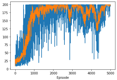
The environment consists of a pole attached to a cart via a joint, with forces that can be applied to the cart in both horizontal directions. The goal is to keep the pole upright (less than 15 degrees from vertical) for as long as possible (while the timesteps are limited to 200 max for this training). The agent receives a reward of +1 for each timestep it keeps the pole from falling over or moving the cart more than 2.4 units away from the center.
Conclusion
Policy Gradient is an efficient Reinforcement Learning (RL) method that does not need to analyze the entire action space, in contrast to previously introduced methods like Q-Learning and thus avoiding the curse of dimensionality.