I am researcher working on robust Military Communication Systems.
Schulman et al. suggest a new policy gradient-based reinforcement learning approach that maintains some of the advantages of trust region proximation optimization (TRPO) while also being much simpler to implement. The general concept involves an alternation between data collection through environment interaction and the optimization of a so-called surrogate objective function using stochastic gradient ascent.
Policy optimization
Policy gradient methods
First of all, since the policy gradient was touched upon in a previous post, it is assumed that the reader is somewhat familiar with the topic. Generally, policy gradient methods perform stochastic gradient ascent on an estimator of the policy gradient. The most common estimator is the following:
$$\hat{g} = \hat{\mathbb{E}}t\left[\nabla\theta\log\pi_\theta(a_t|s_t)\hat{A}_t \right]$$
In this formulation,
\(\pi_\theta\) is a stochastic policy;
\(\hat{A}_t\) is an estimator of the advantage function at timestep $t$;
\(\hat{\mathbb{E}}_t\left[...\right]\) is the empirical average over a finite batch of samples in an algorithm that alternates between sampling and optimization.
For implementations of policy gradient methods, an objective function is constructed in such a way that the gradient is the policy gradient estimator. Therefore, said estimator can be calculated by differentiating the objective.
$$L^{PG}(\theta)=\hat{\mathbb{E}}t\left[\log\pi\theta(a_t|s_t)\hat{A}_t\right]$$
This objective function is also known as the policy gradient loss. If the advantage estimate is positive (i.e., the agent's actions in the sample trajectory resulted in a better-than-average return), the probability of selecting those actions again is increased. Conversely, if the advantage estimate is negative, the likelihood of selecting those actions again is decreased.
Continuously running gradient descent on the same batch of collected experience will cause the neural network's parameters to be updated far outside the range of where the data was originally collected. Since the advantage function is essentially a noisy estimate of the real advantage, it will in turn be corrupted to the point where it is completely wrong. Therefore, the policy will be destroyed if gradient descent is continually run on the same batch of collected experience.
Trust Region Methods
The aforementioned trust region policy optimization algorithm (TRPO) aims to maximize an objective function while imposing a constraint on the size of the policy update (to avoid straying too far from the old policy within a single update), as this would destroy the policy.
$$\begin{align} \max_\theta\,&\hat{\mathbb{E}}t\left[\frac{\pi\theta(a_t|st)}{\pi{\theta_\text{old}}(a_t|s_t)}\hat{A}_t\right] \ \text{subject to }&\hat{\mathbb{E}}t\left[KL\left[\pi{\theta_\text{old}}(\cdot|st), \pi\theta\right]\right]\leq \delta \end{align}$$
Here, \(\theta_{\text{old}}\) is a vector containing the policy parameter before the update.
TRPO suggests using a penalty instead of a constraint because the latter adds additional overhead to the optimization process and can sometimes lead to very undesirable training behavior. This way, the former constraint is directly included in the optimization objective:
$$\max_{\theta}\hat{\mathbb{E}}_t\left[\frac{\pi\theta(a_t|st)}{\pi{\theta_\text{old}}(a_t|st)}\hat{A}t-\beta,KL\left[\pi{\theta\text{old}}(\cdot|st), \pi\theta(\cdot|s_t)\right]\right]$$
That being said, TRPO itself uses a hard constraint instead of a penalty. This is because the introduced coefficient \(\beta\) turns out to be very tricky to set to a single value without affecting performance across different problems.
Therefore, PPO suggests additional modifications to optimize the penalty objective using stochastic gradient descent; choosing a fixed penalty coefficient \(\beta\) will not be enough.
Clipped Surrogate Objective
Say \(r_t(\theta)\) is the probability ratio between the new updated policy and the old policy:
$$rt(\theta) = \frac{\pi\theta(a_t|st)}{\pi{\theta_\text{old}}(a_t|s_t)}$$
$$\Rightarrow \text{ therefore } r(\theta_\text{old})=1.$$
So given a sequence of sampled action-state pairs, this \(r_t(\theta)\) value will be larger than 1 if the action is more likely now than it was in \(\pi_{\theta_{\text{old}}}\). On the other hand, if the action is less probable now than before the last gradient step, \(r_t(\theta)\) will be somewhere between 0 and 1.
Multiplying this ratio \(r_t(\theta)\) with the estimated advantage function results in a more readable version of the normal TRPO objective function, so-called a "surrogate" objective:
$$L^{CPI}(\theta) = \hat{\mathbb{E}}t\left[\frac{\pi\theta(a_t|st)}{\pi{\theta_\text{old}}(a_t|s_t)}\hat{A}_t\right]=\hat{\mathbb{E}}_t\left[r_t(\theta)\hat{A}_t\right]$$
Maximizing this \(L^{CPI}\) without any further constraints would result in a very large policy update, which, as already explained, might end up destroying the policy. Therefore, Schulman et al. suggest penalizing those changes to the policy that would move \(r_t(\theta)\) too far away from 1. Consequently, this is our final result for the final objective:
$$L^{CLIP}(\theta) = \hat{\mathbb{E}}_t\left[\min(r_t(\theta)\hat{A}_t, \text{clip}(r_t(\theta),1-\epsilon,1+\epsilon)\hat{A}_t\right]$$
Basically this objective is a pessimistic bound on the unclipped objective. That is because the objective chooses the minimum between the normal unclipped policy gradient objective \(L^{CLIP}\) and a new clipped version of that objective. The latter discourages moving \(r_t\) outside of the interval \([1 - \epsilon, 1 + \epsilon]\). Two insightful figures are provided in the paper, helping to illustrate this concept.
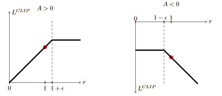
The first graph indicates that, for a single timestep t in \(L^{CPI}\), the selected action had an estimated outcome better than expected. Conversely, the second graph displays an instance when the chosen action resulted in a negative effect on the result. For example, the objective function flattens out for values of r that are too high while the advantage was positive. This means that if an action was good and is now a lot more likely than it was in the old policy update \(\pi_{\theta_\text{old}}\), the clipping prevents too large of an update based on just a single estimate. Again, this might destroy the policy because of the advantage function's noisy characteristics. Of course, on the other hand, for terms with a negative advantage, the clipping also avoids over-adjusting for these values since that might reduce their likelihood to zero while having the same effect of damaging the policy based on a single estimate, but this time in the opposite direction.
If, however, the advantage function is negative and r is large, meaning the chosen action was bad and is much more probable now than it was in the old policy \(\pi_{\theta_\text{old}}\), then it would be beneficial to reverse the update. And, as it so happens, this is the only case in which the unclipped version has a lower value than the clipped version, and it is favored by the minimum operator. This really showcases the finesse of PPO's objective function.
Adaptive KL penalty coefficient
Alternatively or additionally to the surrogate objective proposed by Schulman et al., they provide another concept, the so-called adaptive KL penalty coefficient. The general idea is to penalize the KL divergence and then adapt this penalty coefficient based on the last policy updates. Therefore, the procedure can be divided into two steps:
- First the policy is updated over several epochs by optimizing the KL-penalized objective:
$$L^{KLPEN}(\theta) = \hat{\mathbb{E}}t\left[\frac{\pi\theta(a_t|st)}{\pi{\theta_\text{old}}(a_t|st)}\hat{A}t - \beta KL[\pi{\theta\text{old}}(\cdot|st), \pi\theta(\cdot|s_t)]\right]$$
Then $d$ is computed as \(d = \hat{\mathbb{E}}_t[KL[\pi_{\theta_\text{old}}(\cdot|s_t), \pi_\theta(\cdot|s_t)]]\) to finally update the penalty coefficient \(\beta\) based on some target value of the KL divergence \(d_\text{targ}\):
if \(d<\frac{d_\text{targ}}{1.5}: \beta \leftarrow \beta/2\)
if \(d>d_\text{targ} \times 1.5: \beta \leftarrow \beta\times2\)
This method seems to generally perform worse than the clipped surrogate objective; however, it is included simply because it still makes for an important baseline.
Also note that, while the parameters 1.5 and 2 are chosen heuristically, the algorithm is not particularly sensitive to them and the initial value of \(\beta\) is not relevant because the algorithm quickly adjusts it anyway.
Testing PPO on OpenAI' Gym
To test PPO, the algorithm was applied to several gym environments. Please note that the used implementation of the PPO algorithm originates from OpenAI's stable-baselines3 GitHub repository.
CartPole
This environment might be familiar from previous posts in this series. To quickly summarize, a pole is attached by an unactuated joint to a cart. The agent operates with an action space of two: it can apply force to the left (-1) or the right (+1). The model receives a reward of +1 each timestep if neither of the following conditions are met: the cart's x position exceeds a threshold of 2.4 units in either direction or the pole is more than 15 degrees from vertical; otherwise, the episode ends.

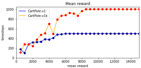
We trained a PPO agent for 15000 timesteps on the environment. The agent reached the perfect mean reward of 500 for CartPole-v1 after only approximately 7500 timesteps of training.
Since gym allows for modification of its environments we created a custom version of CartPole named CartPole-v1k that extends the maximum number of timesteps in an episode from 500 (CartPole-v1) to 1000. Of course this means that the maximum reward for an episode also increased to 1000. As shown in the following figure the PPO agent trained on this new environment reached the maximum reward a little later after about 8500 timesteps.
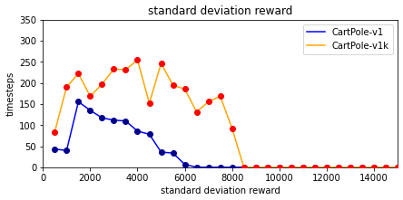
The standard deviation of the reward during the 100 episodes each evaluation step also declines to 0 over even less than the first 8500 timesteps. This means the agent reaches the maximum reward in every single episode after that without fail.
Interestingly, the old model that was trained on the original environment also reached a reward of 1000 on the modified version over all 100 episodes it was evaluated (mean reward of 1000 with a standard deviation of 0). It seems safe to say that the agent not only reached its maximum reward after about 7500 timesteps but also perfected the act of balancing the pole over the next few thousand iterations.
CarRacing
This environment consists of a racing car attempting to maneuver a race track. Observations comprise a 96x96-pixel image, and the action space contains three actions: steering, accelerating, and braking. Each frame is penalized with a negative reward of -0.1, while completion of a track section is rewarded with +1000/N, where N is the number of track sections. Thus, the final reward is calculated as 1000 - the number of frames it took for the agent to complete the track. An episode ends when the car finishes the entire track or moves outside of the 96x96-pixel plane.

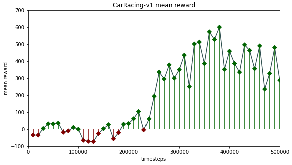
Yet again, we trained a PPO agent--this time over half a million timesteps. Although the mean reward did not fully stabilize over the training period because the agent was still trying out new--and sometimes weaker--strategies, the best model achieved a mean reward of 600 over 50 episodes of evaluation.
This agent was already able to navigate the track and only occasionally oversteered in curves, causing it to lose the track. The following graphic visualizes the 500,000-timestep learning period.
Conclusion
In this post, we have looked at the Proximal Policy Optimization algorithm and its performance on two popular gym environments. We applied PPO to CartPole-v1 and a modified version of it, named CartPole-v1k, where the maximum number of timesteps per episode was increased from 500 to 1000. We trained a separate agent on the Car Racing environment and achieved a mean reward of 600 over 50 evaluation episodes.
PPO is an ideal tool to use with complex, continuous environments such as those discussed in this post. This algorithm operates reliably and efficiently, allowing us to create more sophisticated agents that are capable of outperforming their predecessors. With such powerful reinforcement learning algorithms now available, the possibilities for creating autonomous agents that can successfully interact with their environment are virtually limitless. We look forward to exploring more complex environments and scenarios in future posts.