Reinforcement Learning: Defining Concepts Mathematically
Getting started with Reinforcement Learning!

I am researcher working on robust Military Communication Systems.
This blog post was written in collaboration with my B.Sc. students Jonas Bode, Tobias Hürten, Luca Liberto, and Florian Spelter and is intended to give the reader a baseline understanding of the concepts underlying modern reinforcement learning (RL) algorithms. In particular, this blog post will reintroduce the concepts touched upon in our first blog post, although this time we will use math to build up a repertoire of definitions helping us to understand more advanced concepts and algorithms. Thus our first post is not mandatory to understand RL, yet it is very helpful for newcomers to build up a solid intuition.
The base Concepts
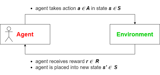
To start off, we will once again begin by examining the agent-environment duality. An RL problem is defined by both the environment and the agent, whose actions affect the related environment. We can now define the interaction of both: given a state \(s \in \mathcal{S}\) it is the agents task to choose an action \(a \in \mathcal{A}\). The environment will then give a reward \(r \in \mathcal{R}\) to the agent and determine the next state \(s' \in \mathcal{S}\) based on the state $s$ and the action $a$ chosen by the agent. While doing so \(\mathcal{S}\) constitutes the set of all possible states, \(\mathcal{A}\) the set of all possible actions, and \(\mathcal{R}\) the set of all possible rewards. The following figure illustrates this relationship.
If we now define \(s_1\) as the starting state and \(r_t, s_t, a_t\) as the state, action or reward at timestep \(t = 1, 2, \ldots, T\) fulfilling the constraint that \(s_T\) is a terminal state, we can define the entire sequence of interactions between agent and environment, also called an episode (sometimes called "trial" or "trajectory"), as follows:
$$ \tau := (s_1, a_1, r_2, s_2, a_2, r_3, \ldots , r_T, s_T) $$
Note that \(s_t, a_t, r_t\) can also be denoted by capital letters \(S_t, A_t, R_t\).
The Environment
The environment can be modeled using a transition function \(P(s', r | s, a)\) representing the probability for transition to $s'$ in the next state and gaining reward $r$, given that the agent choses action $a$ in the present state $s$. Using the transition function we can also derive the state-transition function \(P(s' | s, a)\) as well as the reward function \(R(r | s, a)\):
$$ P(s' | s, a) := P_{s, s'}^a = \sum_{r \in \mathcal{R}} P(s', r | s, a); $$
$$ R(r | s, a) := \mathbb{E} [ r | s, a ] = \sum_{r \in \mathcal{R}} r \sum_{s' \in \mathcal{S}} P(s', r | s, a); $$
where $R$ is the expected value for reward $r$ given state $s$ and action $a$. A single transition can thus be specified by the tuple $(s, a, r, s')$.
Markov Decision Processes
Given an episode \(\tau\) and the transition function \(P(s' | s, a))) we get the following relationship:
$$ s_{t+1} \sim P(s_{t+1} | s_t, a_t) = P(s_{t+1} | s_t, a_t, s_{t-1}, a_{t-1}) = P(s_{t+1} | s_t, a_t, s_{t-1}, a_{t-1},...,s_1, a_1) $$
Therefore, \(s_{t+1}\) only depends on timestep $t$ and the corresponding state-action pair \((s_t,a_t)\). In other words, the future state is independent of the past but depends on the present. This property is also called the Markov Property and enables us to interpret RL problems as Markov Decision Processes (MDPs). While this is not important for elementary algorithms, more advanced approaches utilize this view and its mathematical implications to refine the learning process.
Model-based vs Model-free
Depending on the agent's knowledge about the transition function $P$ and the reward function $R$, we classify RL algorithms as:
- Model-based: The agent knows the environment. This can be further subdivided into:
- Model is given: The agent has complete information regarding $P$ and $R$. AlphaGo can be seen as such an example as the program has complete information regarding the Go rules.
- Model is learned: While $P$ and $R$ are not known in the beginning, the agent learns these functions as part of the learning process.
- Model-free: $P$ and $R$ are neither known nor learned by the agent. Agent57 (the successor of DQN) developed by Google DeepMind falls into this category as the agent plays 57 different Atari games, showing a superhuman performance by learning only using high-dimensional sensory input in form of screen pixels.
The Agent
As stated above, the goal of the agent is to choose the best action $a$ given state $s$. This goal can be formalized using a function \(\pi\), also known as policy. In general the policy can take one of two forms:
- deterministic: \(a = \pi(s)\) (also denoted by \(\mu (s)\)
- stochastic: \(\pi(a | s)\) represents the chance that $a$ is chosen given state $s$. In this case the derived action is denoted by \(a \sim \pi(\cdot | s)\).
As a result, the goal of RL algorithms is to develop a policy \(\pi\) which converges to the optimal policy \(\pi_*\). One of the main differences between algorithms is the method used to determine this policy \(\pi\).
To gain a better understanding of these methods it can be helpful to imagine how a human would go about formulating a strategy in such circumstances. The most intuitive way is to study RL problems using a game-theoretical point of view, meaning that the program effectively replaces a human player.
Value Function
One approach is to assign each state a corresponding value measuring how "good" the state is concerning future rewards. As a result, the strategy becomes to always take the action promising the highest value. This concept is also known as state-value function $V(s)$ (or simply value function).
Yet before we can define $V(s)$ in formal terms, we need to define the future reward also denoted as return \(G_t\) measuring the discounted rewards of an episode:
$$ G_t := r_{t+1} + \gamma r_{t+2} + \gamma^2 r_{t+3} + \ldots = \sum_{k = 0}^\infty \gamma^k r_{t+1+k} $$
The above term for \(G_t\) is called the infinite horizon discounted-return. In comparison, we get the finite horizon discounted-return if the sum is bounded by a finite parameter $T$.
Here, \(\gamma \in [0, 1]\) is a hyperparameter discounting future rewards by their distance. Using \(\gamma\) has multiple practical reasons, as we may prefer immediate benefits over drawn-out ones (such as winning a game quickly). Furthermore, this provides mathematical advantages when encountering loops in the transition sequence. As a result, we can define \(G_t\) as follows:
$$ G_t = r_{t+1} + \gamma r_{t+2} + \gamma^2 r_{t+3} + \ldots $$ $$ = r_{t+1} + \gamma (r_{t+2} + \gamma r_{t+3} + \ldots) $$ $$ = r_{t+1} + \gamma G_{t+1} $$
Now, using the return \(G_t\) we can define $V(s)$ as:
$$ V(s) := \mathbb{E}[G_t | s_t = s] $$ $$ V_\pi(s) = \sum_{a} \pi(a | s) \sum_{s', r} P(s', r | s, a) (r + \gamma V_\pi(s')) $$
Note the dependency of $V(s)$ on the episode or policy.
The second equation here is also called the Bellman equation. Therefore, a policy is required to determine the state-value function and we can define \(V_{\ast}\) to be the function generated by the optimal policy \(\pi_*\). In sequence, if $V(s)$ is given we can derive a greedy policy \(\pi\) :
$$ \pi(s) = \arg \max_{a} \sum_{s', r} P(s', r | s, a) (r + \gamma V(s')) $$
In other words, if we can state an algorithm computing $V(s)$ such that it converges to \(V_{\ast}\), then this yields an optimal policy \(\pi_{\ast}\). This is the idea behind the policy-iteration algorithm, which alternates between generating a state-value function from a given policy and generating a policy using the state-value function.
Action-Value Function
Another possibility is to evaluate state-actions pairs, resulting in the action-value function $Q(s, a)$. To this end, we define $Q(s, a)$ in a similar fashion and connect both functions $Q(s, a)$ and $V(s)$ for a given policy:
$$ Q(s, a) := \mathbb{E}[G_t | s_t = s, a_t = a] $$
$$ V_\pi(s) = \sum_{a} \pi(a | s) Q_\pi(s, a) $$
$$ Q_\pi(s, a) = \sum_{s', r} P(s', r | s, a) (r + \gamma V_\pi(s')) $$
In this case, the Bellman equation is defined as:
$$ Q_\pi(s, a) = \sum_{s', r} P(s', r | s, a) (r + \gamma \sum_{a'} \pi(a' | s) Q_\pi(s', a')) $$
And the action-value function can also be used to generate a greedy policy:
$$ \pi(s) = \arg \max_{a} Q(s, a) $$
Approaches to Reinforcement Learning
In theory, every problem solved using this framework can be interpreted as a simple planning problem, aiming to find an optimal solution to the Bellman equation, thus determining an optimal policy. In practice, however, the number of possible states and actions as well as the limited knowledge of the environment makes this approach unfeasible, thus enforcing us to find another way of computing the optimal policy. Therefore, algorithms tend to optimize the state-value function, the action-value function, or the policy using a straightforward approach. If the policy is optimized straightforward, we can describe the policy using a precise analytical function and solve the problem by optimizing a given set of parameters. This is what we describe in the following blog posts.
Since we have defined the most important terms, let us go more deeply into specific algorithms and approaches in the following posts.